Synthetic music video: kiriloff – Fortschritt
A synthesized music video of the piece “Fortschritt” from kiriloff programmed in Python. It uses aubio for onset detection in the audio signal. Input video clips are alienated by drawing Voronoi diagrams derived from a sample of feature points from a binarized frame of the input clip. Video rendering is done with MoviePy and synthetic frame generation uses Gizeh and cairocffi.
The code is also on github.
Inspiration
The following blog posts inspired me to make this music video:
Further explanation on synthetic frame rendering
The synthetic frames are generated using the following (very simplified) pipeline implemented in a script that uses MoviePy for video editing:
1. Inputs
We have an original input clip frame C at a certain time t:

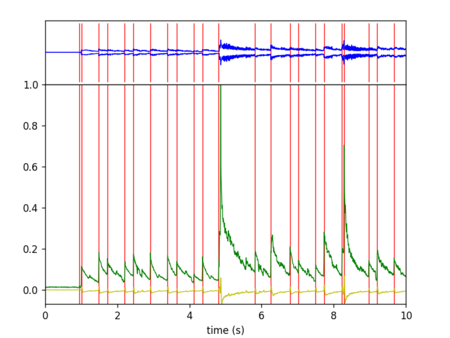
Additionally, we have the onset amplitude O at t. The onset amplitude is the “strength” of a detected note at this time. For example, you can see in this image the detected onsets as red bars and the amplitude as green line. Both are combined by finding the maximum amplitude between to onsets to get the onset amplitude.
2. Binarization and feature generation
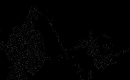
C is first blurred with a kernel size 5 in order to reduce noise and then binarized using Otsu’s method. Both is done using OpenCV. We get the following picture:

From the binarized image, we generate features F (the coordinates in frame image space where the binarized image is white), i.e. we get a list [(x1, y1), (x2, y2), ... (xn, yn)] where x and y are coordinates of the white pixels in the above image. For example in the above image, we get almost 500,000 features, i.e. there are almost 500,000 white pixels in the above image.
3. Sampling
Sample from F according to O (i.e. the higher the onset amplitude the more features get sampled and the more Voronoi cells will be drawn) to get S. See the following picture where 6000 random points were sampled from the almost 500,000 features of the binarized image:
(Note that the sampled white pixels are hardly visible because they are very small as the resolution of the frame is quite high)
4. Create Voronoi regions
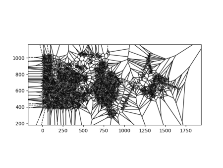
From feature samples S the Voronoi regions are calculated using SciPy’s Voronoi class. The raw SciPy plot looks like this:
5. Calculate Voronoi cell lines and draw them
The lines that make up the borders between the Voronoi regions are calculated to get to a Voronoi diagram restricted to frame image space. These lines are drawn according to scene definitions either with a solid color or with a color gradient using start and stop colors from the pixels of both end points of the line in the input clip. This for example draws the Voronoi cells on a white background and uses the color gradient effect:
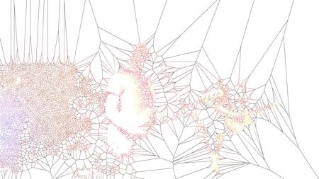
Note that the actual rendering pipeline is little more complex as it also draws Voronoi diagrams of previous frames with decreasing transparency over time to get a smooth “changing spider webs” effect.
← Back